Simulating vaterite with DDA

This section is a companion for the examples/dda_vaterite.m script and will guide you through simulating an inhomogeneous particle using the discrete dipole approximation. The script simulates the vaterite particles described in

Highly birefringent vaterite microspheres: production, characterization and applications for optical micromanipulation. S. Parkin, et al., Optics Express Vol. 17, Issue 24, pp. 21944-21955 (2009) https://doi.org/10.1364/OE.17.021944

These particles are made of a uniaxial birefringent material. The crystal axis is aligned according to a sheaf-of-wheat structure, shown in figure Fig. 6. In order to simulate this particle, we need to specify the polarizability of each dipole (computational unit cell).

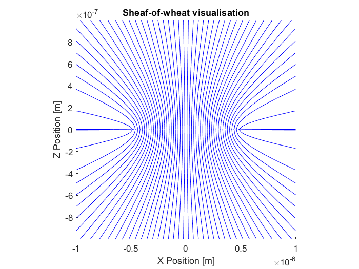
Fig. 6 Illustration of the vaterite sheaf of wheat structure. The image shows a slice through the XZ plane. The particle is rotaionly symmetry about the Z axis and mirror symmetric about the XY plane.

Describing the vaterite properties

To describe the vaterite shape, we use ott.shapes.Sphere. DDA requires the shape to be specified using voxels, for this we used ott.shapes.Sphere.voxels() to calculate voxels on a grid with a regular spacing.

spacing = wavelength0 / 10;
radius = wavelength0;
shape = ott.shapes.Sphere(radius);
voxels = shape.voxels(spacing, 'even_range', true);

The even_range parameter tells the voxels function to use an even number of points for the size of each voxel grid dimension. This means that the voxel grid will not place voxels at the origin making it easier to use mirror and rotational symmetry options for DDA.

To calculate the polarizability for a unit cell we use the method based on the lattice dispersion relation from ott.utils.polarizability. Vaterite is a uniaxial crystal with an ordinary and extraordinary refractive index, index_o and index_e respectively.

upol = ott.utils.polarizability.LDR(spacing ./ wavelength0, ...
   [index_o; index_o; index_e] ./ index_medium);

To generate the sheaf of wheat structure we used the sheafOfWheat function defined in the script to calculate the orientation direction of each unit cell.

dirs = sheafOfWheat(voxels, 0.5*radius);

Finally, we rotate the polarisability and refractive index so the z direction aligns with the sheaf-of-wheat direction

index_relative = ott.utils.rotate_3x3tensor(...
    diag([index_o, index_o, index_e] ./ index_medium), 'dir', dirs);
polarizabilities = ott.utils.rotate_3x3tensor(...
    diag(upol), 'dir', dirs);

Calculating the T-matrix with DDA

Once all the properties have been described, we construct the T-matrix using ott.TmatrixDda. We use the class constructor rather than ott.TmatrixDda.simple() in order to specify the polarizability of each voxel. If we wanted to simulate a homogeneous sphere we could use the simple method.

Tmatrix = ott.TmatrixDda(voxels, ...
     'polarizability', polarizabilities, ...
     'index_relative', index_relative, ...
     'index_medium', index_medium, ...
     'spacing', spacing, ...
     'z_rotational_symmetry', 4, ...
     'z_mirror_symmetry', true, ...
     'wavelength0', wavelength0, ...
     'low_memory', low_memory);

Most of the arguments are fairly intuitive: we specify the material properties and voxel locations with voxels and polarizabilities. When polarizabilities are specified explicitly, we still need to specify index_relative in order to ensure correct scaling of the resulting T-matrix. The z_rotational_symmetry argument tells the DDA implmenetation to use fourth order rotational symmetry about the z-axis and the z_mirror_symmetry says to use mirror symmetry about the XY plane. The low memory option can be used with rotational symmetry or mirror symmetry to reduce the amount of memory required at a slight reduction to computational efficiency. spacing is currently only used for the Nmax estimation. If the polarizabilities were not specified, spacing would also be used for calculating the polarizabilities from index_relative. wavelength0 and index_medium specify the units for distance, i.e. the scaling that should be applied to voxels.

Depending on the size of the particle and the number of dipoles, this could take anywhere from a couple of minutes to several hours to run. An alternative is to only calculate modes which are present in the illuminating beam, this can be achieved using the modes option, for examples, to a beam with only m = 1 modes you could do

Nmax = 5;
m = 1;
n = max(1, abs(m)):Nmax;
modes = [n(:), repmat(m, size(n(:)))];

Tmatrix = ott.TmatrixDda(voxels, ...
   'modes', modes);

The above could also be used to calculate the T-matrix in parallel by specifying a different mode for each worker to calculate and then combining the T-matrix columns after calculation.

If you are calculating large T-matrices, you will probably want to save them to a file so you can use them again later without needing to rerun DDA. For this, simply use the save command

save('output.mat', 'Tmatrix')

To load the T-matrix back into Matlab, first make sure OTT is on the matlab path and then either double click on the .mat file or run

load('output.mat')

Calculating torque on the particle

The calculated T-matrix can be used like any other T-matrix object. For example, we can create a beam and calculate the torque on the particle at different locations in the beam:

beam = ott.BscPmGauss('NA', 1.1, 'index_medium', index_medium, ...
   'power', 1.0, 'wavelength0', wavelength0, 'polarisation', [1, -1i]);

[~, tz] = ott.forcetorque(beam, Tmatrix, ...
    'position', [0;0;0], 'rotation', eye(3));