Calculating forces on a spherical particle
This section is a companion for the examples/example_sphere.m script
and will guide you through the core functionality of the toolbox.
The script sets up the variables for calculating forces on a spherical
particle in a Gaussian beam. The particle is created using the
ott.Tmatrix.simple() method, which for a spherical particle
calls the ott.TmatrixMie class constructor.
The beam is constructed using the ott.BscPmGauss class which
can also be used for Laguerre-Gaussian and Hermite-Gaussian beam modes.
And, forces are calculated using ott.forcetorque().
A similar example is described in Calculating forces with the GUI.
Contents
Setting up the Matlab workspace
The example_sphere.m script starts by setting up the Matlab workspace
to work with OTT.
The first step is to add OTT to the Matlab path, this step is not required
if OTT is already on the path (for instance, if you installed OTT via the
add-ons menu, OTT should already be on the path).
addpath('../'); % Change this to your OTT path if required
The next step is clearing all existing variables and configuring OTT specific warnings. Some OTT functions can trigger many warnings, to reduce the verbosity of the output, OTT can be asked to only warn once about issues during this Matlab session. Several OTT functions are also likely to move in a future release, we can turn off warnings related to these changes here too.
close all;
ott.warning('once');
ott.change_warnings('off');
Next, we declare our material properties, wavelength, sphere radius and numerical aperture for the objective.
n_medium = 1.33;        % Water
n_particle = 1.59;      % Polystyrene
wavelength0 = 1064e-9;  % Vacuum wavelength
wavelength_medium = wavelength0 / n_medium;
radius = 1.0*wavelength_medium;
NA = 1.02;              % Numerical aperture of beam
Generating the beam shape coefficients
To create a beam, we use ott.BscPmGauss.
The constructor for this class accepts several positional and named
arguments, in this example we set the numerical aperture, polarisation,
refractive index and vacuum wavelength.
beam = ott.BscPmGauss('NA', NA, 'polarisation', [ 1 1i ], ...
     'index_medium', n_medium, 'wavelength0', wavelength0);
The class can also be used for generating Laguerre-Gaussian beams and other type of beams by adding additional parameters. For example, the following would generate an LG(0, 3) beam
beam = ott.BscPmGauss('lg', [ 0 3 ], ...
     'polarisation', [ 1 1i ], 'NA', NA, ...
     'index_medium', n_medium, 'wavelength0', wavelength0);
We may also want to set or normalise the beam power, this can be done at
any time by setting the power property, for example
beam.power = 1.0;
Regardless of the type of beam we are using, we are now able to visualise
the beam. The ott.Bsc base class (which ott.BscPmGauss
inherits from) defines several visualisation function.
To visualise the field around the focus, we can use
ott.Bsc.visualise(). Before calling the function we need to
specify the vector spherical wave function basis to use, for near-field
visualisation this should be set to regular.
beam.basis = 'regular';

figure();
subplot(1, 2, 1);
beam.visualise('axis', 'y');
subplot(1, 2, 2);
beam.visualise('axis', 'z');
The above code should produce something similar to figure Fig. 2. The axis parameter specifies which axis should be normal to our visualisation slice.
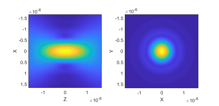
Fig. 2 Visualisation of the incident beam near-field.
We can also visualise the far-field of the beam.
For this we set the basis to incoming and use the
ott.Bsc.visualiseFarfield() function.
beam.basis = 'incoming';

figure();
beam.visualiseFarfield('dir', 'neg');
The above should produce something similar to figure Fig. 3. The dir parameter specifies which hemisphere we want to look at, in this case we look at the negative (backward) hemisphere. Depending on the beam and the chosen basis, either the forward or backward hemisphere may have very little power, if you are unsure about the direction of your beam it is a good idea to look in both directions.
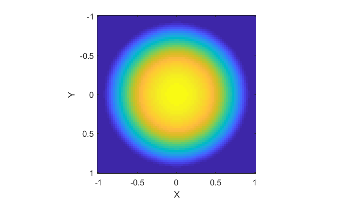
Fig. 3 Visualisation of the incident beam far-field.
Generating the T-matrix
In this simulation we use a T-matrix for a spherical particle.
The T-matrix is diagonal and the elements along the diagonal are
the Mie coefficients for a sphere.
To calculate the T-matrix we use the ott.Tmatrix.simple()
method, we specify the shape as a sphere and the method automatically
selects the best method for this shape, in this case
ott.TmatrixMie.
The ott.Tmatrix.simple() method takes various named parameters
for the particle size, shape and refractive index.
T = ott.Tmatrix.simple('sphere', radius, 'wavelength0', wavelength0, ...
   'index_medium', n_medium, 'index_particle', n_particle);
For a sphere, this should only take a couple of seconds to evaluate.
Calculate the scattered field
The T-matrix and beam objects encapsulate the data for the T-matrix
and beam shape coefficients (a matrix and vector respectively).
We can view this data by accessing the data attribute of these objects,
for example
disp(T.data);
In the T-matrix method, a T-matrix describes how a particle scatters light. It is a linear matrix which relates each incident mode to each scattered mode, mathematically this is
where \(T\) is the T-matrix, and \((a,b)\), \((p, q)\) are the incident and scattered beam shape coefficients. To implement this in OTT, we can simply write
sbeam = T * beam;
This is equivalent to directly multiplying the
T.data and beam.data matrix and vector objects to calculate
the resulting scattered beam shape coefficients, and encapsulating
the result in a ott.Bsc object.
As with the incident beam, we are able to generate various visualisations of the fields. The following example shows a visualisation of the scattered field and the total field (incident + scattered) around the beam focus, for the sphere and Gaussian beam described above, the results are shown in Fig. 4.
figure();
subplot(1, 2, 1);
sbeam.basis = 'outgoing';
sbeam.visualise('axis', 'y', ...
   'mask', @(xyz) vecnorm(xyz) < radius, 'range', [1,1]*2e-6)
title('Scattered field');

subplot(1, 2, 2);
tbeam = sbeam.totalField(beam);
tbeam.basis = 'regular';
tbeam.visualise('axis', 'y', ...
   'mask', @(xyz) vecnorm(xyz) < radius, 'range', [1,1]*2e-6)
title('Total field');
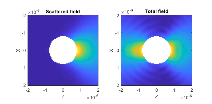
Fig. 4 The total and scattered field visualised for a spherical particle at the focus of a Gaussian beam. This slice is along the beam axis, the region corresponding to the particle has been removed.
The T-matrix in this example only gives the fields outside the particle,
we use the mask parameter to remove the region inside the particle.
To visualise the fields inside the particle we would need to calculate
a internal T-matrix instead.
Calculating optical forces
Now that we have a scattered beam, we are able to calculate the change
in momentum between the incident beam and the particle; and, therefore,
infer the force acting on the particle.
The main function for calculating forces is ott.forcetorque(),
this function can operate on beams or beams and T-matrix.
When both the inputs are beams, the function calculates forces and
torques using various summations over the beam shape coefficients.
[force, torque] = ott.forcetorque(beam, sbeam);
In this example, the force would be 0.0135 and the torque would be
1e-16 which is on the order of round-off error (i.e. numerically
equivalent to zero).
The units depend on the units used for the beam, in this example we
can convert to SI units (Newtons) using
nPc = 0.001 .* index_medium / 3e8;  % 0.001 W * n / vacuum_speed
force_SI = force .* nPc
Beam translations
Being able to calculate optical forces is only useful if we can
translate either the beam or the particle to different locations.
For this, we can use the beam ott.Bsc.translateXyz() function.
The behaviour of this function depends on the current beam basis:
if the beam was generated using one of the ott.Bsc* functions,
the basis should typically be set to regular; if the beam was generated
from scattering by another particle, the basis should be outgoing.
For example, in this example we could translate the beam along the
x-axis with
beam.basis = 'regular';
x = 1.0e-6; y = 0.0e-6; z = 0.0e-6;
offset_beam = beam.translateXyz([x; y; z]);
We could translate the beam and calculate the forces multiple times
with the above method; however, OTT provides a more convinient method
using ott.forcetorque().
Calculate multiple forces with ott.forcetorque
Instead of passing two beam objects to ott.forcetorque(), we could
instead pass a beam and T-matrix object and the various positions
we want to translate the beam to.
As with other translations, it is important to set the basis of the
incident beam before calling the method.
The following code calculates the force along the beam axis (the
z-axis), output is shown in Fig. 5.
xyz = [0;0;1] .* linspace(-4, 4, 100).*1e-6;
fxyz = ott.forcetorque(beam, T, 'position', xyz);

figure();
nPc = n_medium / 3e8;  % n / vacuum_speed
plot(xyz(3, :), fxyz .* nPc);
xlabel('Z position [m]');
ylabel('Force [N/W]');
legend({'Fx', 'Fy', 'Fz'});
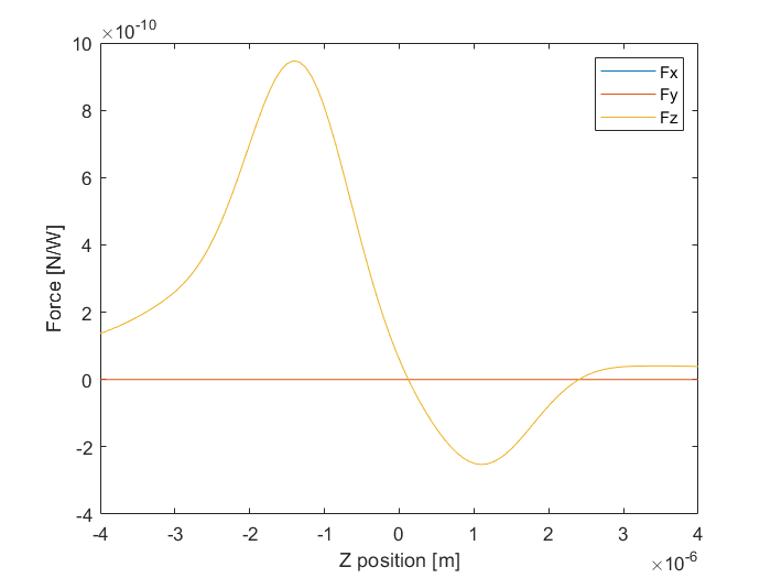
Fig. 5 The force on a spherical particle positioned at different locations along the beam axis. The transverse components of the force are approximately zero. The axial force displays the well known profile of an optically traped particle.